haloR - A New R Halo API Wrapper
Earlier this week Microsoft released Halo Wars 2, a followup to the original that has somewhat of a cult following. In contrast to the mainline Halo titles, Halo Wars is a real-time strategy game. I've played through the Halo Wars 2 campaign and dipped my feet a little bit into the multiplayer. It isn't really for me (I prefer FPS) but it was still an enjoyable experience.
Similar to Halo 5, Microsoft and 343i have decided to open up much of the game details to the public through their Halo API. I really enjoyed digging through Halo 5 data and it was a big engagement point for my interest in the game. Kudos to MS/343i for the work they do on this stuff.
Even though I don't plan to continue playing the game, I decided to update my Halo R API wrapper to now include functions to easily get data from the Halo Wars 2 endpoints. Installation instructions and a tiny example can be found on the haloR Github.
Before using it, I suggest reading through the documentation provided my 343i since the documentation for my package is kind of sparse and the returned objects can be a little bit cryptic without a reference.
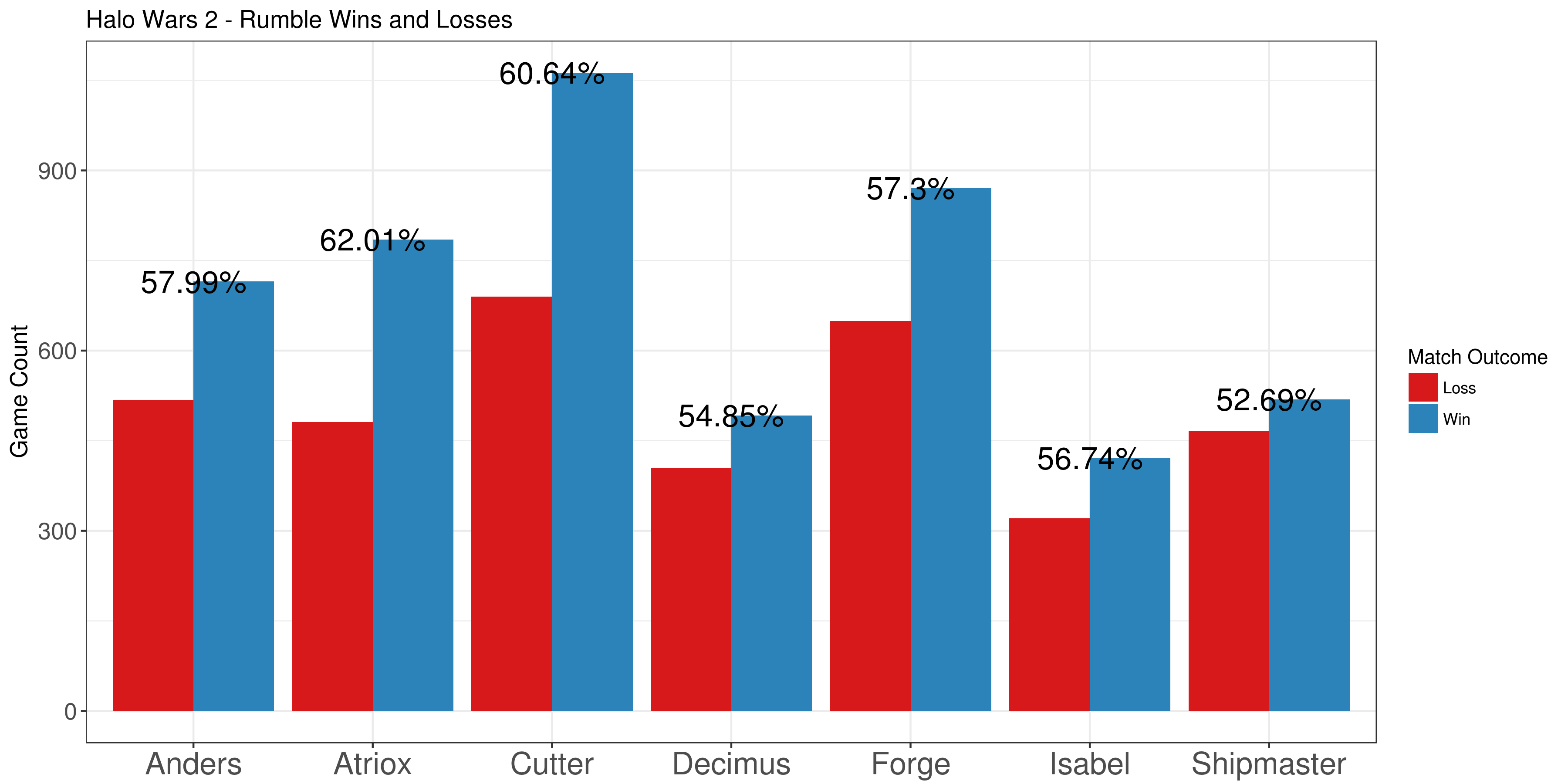
And as an additional small example, I pulled some Halo Wars 2 data for the game mode 'Rumble'. This is a new mode where players have infinite resources and don't have to worry about their economy. I wanted to see which leader had the highest winrates so I pulled a bunch of matches and graphed their percentages (at the top of this post). It's interesting that the two main story characters, Cutter and Atriox, have the highest winrates.
Simple Regression Trees in Julia
Being a data analyst, it’s a bit embarrassing how little experience I have with the new hotness of machine learning. I recently had a conversation with an individual who mentioned that they often employ decision and regression trees as a data exploration method and this prompted me to start looking into them.
Decision and regression trees are an awesome tool because of how transparent the end result is. It’s easy to understand and to explain to others who might be weary of implementing something opaque. In the simplest trees, they ask a series of yes-no questions such as: is a certain variable greater than some number. With each question you progress through different paths until you reach a terminal node. This terminal node will give you a prediction, either a classification or a value, depending on the type of tree. This process is extremely easy to follow and is the biggest selling point of decision trees.
Another advantage of decision trees is the simplicity of the algorithm used to create the tree. There are 3 basic steps that go into creating a tree. The first is a calculation on some cost function that we want to minimize. In the case of regression trees the cost function is usually just the mean squared error of all observations at that particular node. Secondly, each variable is iterated over to find the optimal way to divide the observations into two groups. Optimal, in this case, refers to the smallest mean squared error. And finally, once the optimal division is found the process is repeated on the two subgroups. This continues until certain predefined conditions are reached like minimum number of observations at a node.
In fact, the algorithm is so simple I decided to implement a basic regression tree in Julia as a learning exercise. Julia is an awesome statistical computing language thats main advantage is speed. Code written in Julia is often several times faster than the equivalent R or Python code for non-trivial calculations. My implementation is rather limited compared to the ‘rpart’ package in R or even the ‘DecisionTrees.jl’ package available in Julia. The idea was to gain a better understanding of how decision trees actually work and not to replace any of the already great implementations available.
I tested my implementation on the 'cu.summary' dataset from 'rpart'. This dataset contains information on a small number of cars and regressing on mileage gives the following tree:
Price < 9415.84 : 1
  Price < 6696.9 : 2
    4 : 34.0 : 3
    7 : 30.714285714285715 : 3
  Type IN String["Small","Sporty","Compact"] : 2
    Price < 11475.8 : 3
      Reliability IN String["average","Much worse"] : 4
        4 : 27.25 : 5
        6 : 24.166666666666668 : 5
      Reliability IN String["Much worse","better"] : 4
        4 : 21.0 : 5
        7 : 24.428571428571427 : 5
    Type IN String["Medium"] : 3
      Reliability IN String["Much better","worse"] : 4
        6 : 21.333333333333332 : 5
        5 : 22.2 : 5
      6 : 19.333333333333332 : 4
The labels show the decision that is made at each node. The lines that begin with a number show the number of observations that were placed in that bin along with the average mileage of those observations. The output isn’t pretty but it isn’t that difficult to follow since the tree is pretty shallow.
And, as always, I’ve uploaded my code to Github.

