Earlier this week Microsoft released Halo Wars 2, a followup to the original that has somewhat of a cult following. In contrast to the mainline Halo titles, Halo Wars is a real-time strategy game. I've played through the Halo Wars 2 campaign and dipped my feet a little bit into the multiplayer. It isn't really for me (I prefer FPS) but it was still an enjoyable experience.

Similar to Halo 5, Microsoft and 343i have decided to open up much of the game details to the public through their Halo API. I really enjoyed digging through Halo 5 data and it was a big engagement point for my interest in the game. Kudos to MS/343i for the work they do on this stuff.

Even though I don't plan to continue playing the game, I decided to update my Halo R API wrapper to now include functions to easily get data from the Halo Wars 2 endpoints. Installation instructions and a tiny example can be found on the haloR Github.

Before using it, I suggest reading through the documentation provided my 343i since the documentation for my package is kind of sparse and the returned objects can be a little bit cryptic without a reference.

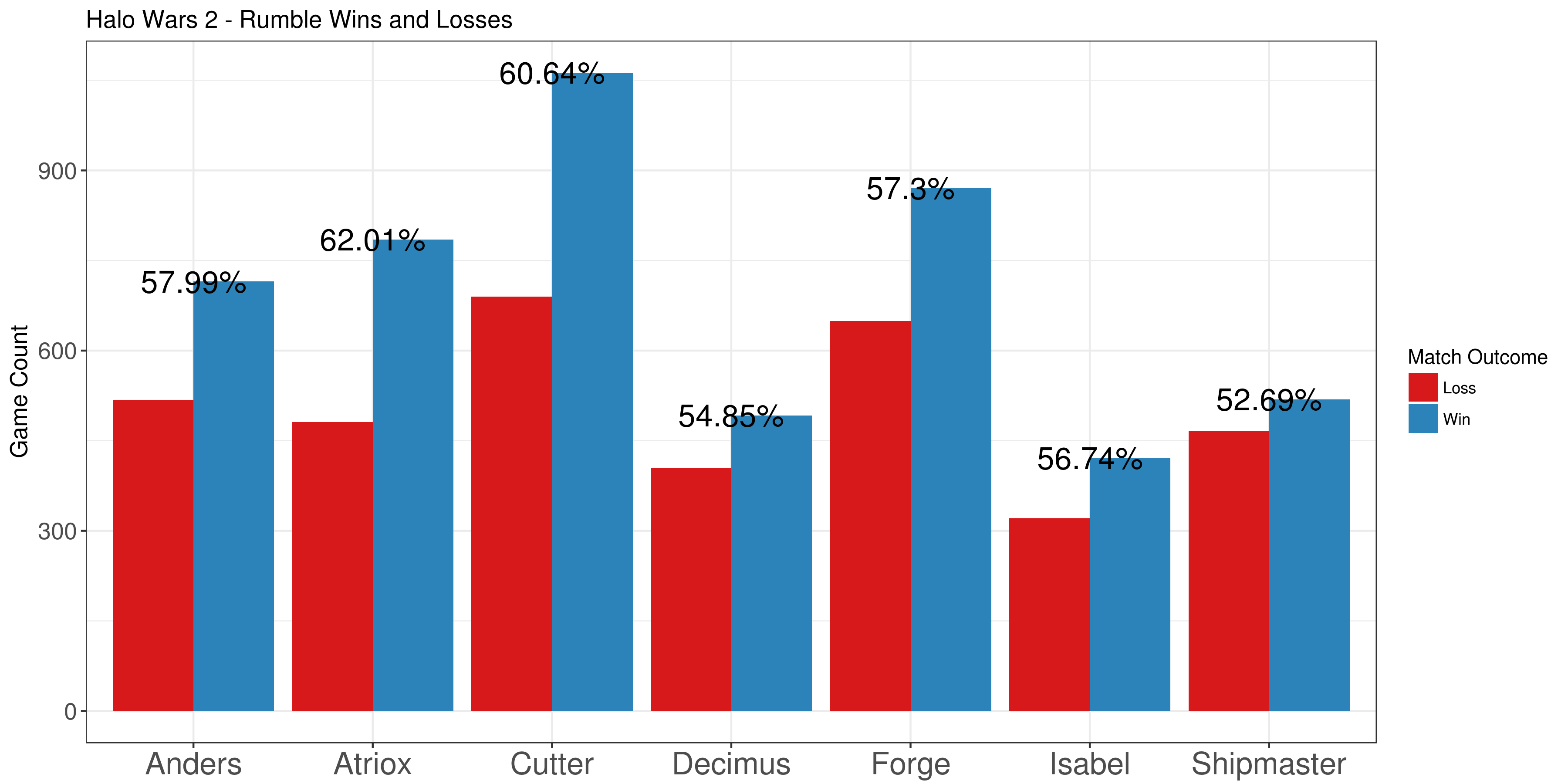
And as an additional small example, I pulled some Halo Wars 2 data for the game mode 'Rumble'. This is a new mode where players have infinite resources and don't have to worry about their economy. I wanted to see which leader had the highest winrates so I pulled a bunch of matches and graphed their percentages (at the top of this post). It's interesting that the two main story characters, Cutter and Atriox, have the highest winrates.

Being a data analyst, it’s a bit embarrassing how little experience I have with the new hotness of machine learning. I recently had a conversation with an individual who mentioned that they often employ decision and regression trees as a data exploration method and this prompted me to start looking into them.

Decision and regression trees are an awesome tool because of how transparent the end result is. It’s easy to understand and to explain to others who might be weary of implementing something opaque. In the simplest trees, they ask a series of yes-no questions such as: is a certain variable greater than some number. With each question you progress through different paths until you reach a terminal node. This terminal node will give you a prediction, either a classification or a value, depending on the type of tree. This process is extremely easy to follow and is the biggest selling point of decision trees.

Another advantage of decision trees is the simplicity of the algorithm used to create the tree. There are 3 basic steps that go into creating a tree. The first is a calculation on some cost function that we want to minimize. In the case of regression trees the cost function is usually just the mean squared error of all observations at that particular node. Secondly, each variable is iterated over to find the optimal way to divide the observations into two groups. Optimal, in this case, refers to the smallest mean squared error. And finally, once the optimal division is found the process is repeated on the two subgroups. This continues until certain predefined conditions are reached like minimum number of observations at a node.

In fact, the algorithm is so simple I decided to implement a basic regression tree in Julia as a learning exercise. Julia is an awesome statistical computing language thats main advantage is speed. Code written in Julia is often several times faster than the equivalent R or Python code for non-trivial calculations. My implementation is rather limited compared to the ‘rpart’ package in R or even the ‘DecisionTrees.jl’ package available in Julia. The idea was to gain a better understanding of how decision trees actually work and not to replace any of the already great implementations available.

I tested my implementation on the 'cu.summary' dataset from 'rpart'. This dataset contains information on a small number of cars and regressing on mileage gives the following tree:

Price < 9415.84 : 1
  Price < 6696.9 : 2
    4 : 34.0 : 3
    7 : 30.714285714285715 : 3
  Type IN String["Small","Sporty","Compact"] : 2
    Price < 11475.8 : 3
      Reliability IN String["average","Much worse"] : 4
        4 : 27.25 : 5
        6 : 24.166666666666668 : 5
      Reliability IN String["Much worse","better"] : 4
        4 : 21.0 : 5
        7 : 24.428571428571427 : 5
    Type IN String["Medium"] : 3
      Reliability IN String["Much better","worse"] : 4
        6 : 21.333333333333332 : 5
        5 : 22.2 : 5
      6 : 19.333333333333332 : 4

The labels show the decision that is made at each node. The lines that begin with a number show the number of observations that were placed in that bin along with the average mileage of those observations. The output isn’t pretty but it isn’t that difficult to follow since the tree is pretty shallow.

And, as always, I’ve uploaded my code to Github.

Building a clock with nixie tubes is a project that has been done to death already. A quick google search will yield thousands of variants put together by just as many different people. So even though it’s not the most original project, nixie tubes have such a cool look to them I had to make my own anyway. I think the warm glow always catches people’s eye with a look that is somehow both futuristic and retro at the same time.

There were a couple goals that I set for the project. Firstly, I wanted to design as much of the clock as I could. This was made pretty easy by the sheer amount of information available online. As I said, thousands of people have attempted this already and there is no shortage of documentation. The tubes themselves are salvaged IN-14 style tubes produced in the Soviet Union. They even have the CCCP logo printed on the backs of a couple that haven’t yet worn away.

I used the site EasyEDA to design the schematic and PCB board layout. I got the PCB fabricated from there as well and they turned out pretty nice. Although the minimum I could order was 6 so I got a few extras that I’m not sure what to do with. It was cool to design my own board and layout everything the way I wanted it. I had never done any CAD stuff before so it was a fun experience.

Another thing I really wanted for the clock was accurate timekeeping. I found that using the internal clock from the Arduino was pretty inaccurate as over time it would fluctuate for many different reasons. Another option was to use a real-time clock chip, like those in digital watches. But I decided against it because even watches can drift by a minute or two over several months. The final option, and the one I went with, was to use a GPS chip. Going with GPS means that the clock will always have exactly GMT time, as provided by the satellites. Which means I only have to adjust the hour instead of setting the whole time when resetting it. Of course, if you live somewhere strange, like Newfoundland with a half timezone, the minutes will still need to be adjusted too.

My board design is uploaded here if you'd like to take a look or get your own fabricated.
And the Arduino code is, as always, on my Github.

If you've been on the internet over the past couple of weeks then you've likely heard of the so-called Dirty COW bug recently discovered in Linux. The story behind it is actually kind of funny. It was discovered and patched by Linus himself over 11 years ago! The fix was then undone in subsequent code commits due to issues with new code. So the vulnerability has been exploitable since for about 9 years, since 2007. The silver lining is that no examples of this exploit being used have been found in the wild and most popular Linux distros have pushed fixes. Patch your system if you haven't already!

If you're not familiar with what dirty COW does it allows a non-privileged user to write to files that are usually read-only except by root. This is pretty significant and since "everything in Unix is a file" this opens up lots of doors for exploitation. There are plenty of resources online to learn more about how exactly the exploit works, like here, so I won't go into much detail about the exploit itself.

Along with knowledge of the exploit, proof-of-concept code was also released. Basically a skeleton example with just enough code to show how writing to a root-protected file is possible. This is what I used to create a simple command line program that I call Madcow. It takes advantage of the dirty COW exploit to change the root password on an Ubuntu system to whatever the user provides.

Ubuntu stores passwords (sort of) in a file located at '/etc/passwd'. Here is the first couple lines of the one found on my machine:

root:x:0:0:root:/root:/bin/bash

daemon:x:1:1:daemon:/usr/sbin:/usr/sbin/nologin

bin:x:2:2:bin:/bin:/usr/sbin/nologin

sys:x:3:3:sys:/dev:/usr/sbin/nologin

sync:x:4:65534:sync:/bin:/bin/sync

games:x:5:60:games:/usr/games:/usr/sbin/nologin

This file is read-only to all users except root. There's lots of stuff here but the most important information is after the first colon of each line. Right at the top we see 'root' then a colon, a lowercase 'x', and another colon. There can be two types of information here: an encrypted password (storing plaintext passwords in files readable by all users would be silly), or a lowercase 'x'. The lowercase 'x' indicates that the encrypted version of the password is stored in a separate file '/etc/shadow'. That file is readable only by root so changing it is impossible.

So if we want to change the root password all we need to do is replace the single lowercase 'x' with an encrypted password of our choosing. And this is exactly what madcow does. Here is a quick example:

$ head -1 /etc/passwd

       root:x:0:0:root:/root:/bin/bash

$ ./madcow new_password

       mmap 7f4b13aba000

       madvise 0

       procselfmem 2648940

$ head -1 /etc/passwd

       root:xxTumM4gi9IDM:0:0:root:/root:/bin/bash

Not very interesting on the surface, but this is a write-protected file that we, as a normal user, have just written to! Now it's simply a matter of starting a root shell using the new password and the entire system is ours.

That's basically it. I'm sure there are a lot more interesting things that could be done with this exploit but this is the most obvious and powerful. The code is available on my Github if you want to take a closer look. Obviously I take no responsibility for any damage caused to your or others' systems from running this code. And please don't run it outside of a VM or an installation you don't mind losing.

The more I play around with Julia the better things seem to get. With web-stuff on my mind lately from working on MiniHTTP I thought it would be cool to create a simple web API for adding charts to any webpage. Thanks to a couple packages (HttpServer.jl and Plots.jl) this was dead easy in Julia.

The basis for handling requests for charts is by creating a simple HTTP Handler. This checks the URL that was supplied and, if it matches, dispatches the correct chart.

http = HttpHandler() do req::Request, res::Response
  if ismatch(r"^/randomchart",req.resource)
    Response(random_chart(), headers("image/png"))
  elseif ismatch(r"^/linechart",req.resource)
    Response(line_chart(req.resource), headers("image/png"))
  else
    Response(400)
  end
end

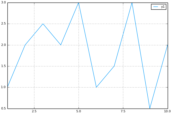
Above there are two endpoints that we can match. The first one is if the URL starts with ‘/randomchart’, in this case the function ‘random_chart()’ is called which generates some random numbers and plots them to a chart. The chart at the top of this post in made this way and, since it is random, every time this page is refreshed the chart will be slightly different.

The second endpoint is for generating a custom line chart. If the URL starts with ‘/linechart’ then the function ‘line_chart(::AbstractString)’ is called. This function expects that a query string is attached to the end of the supplied URL that contains a list of x and y coordinates to plot on a line graph. For instance, the URL ‘/linechart?x=1,2,3,4,5,6,7,8,9,10&y=1,2,2.5,2,3,1,1.5,3,0.5,2’ was used to generate the plot below.

And that’s really all there is to it. The full code (which is less than 50 lines!) has been uploaded to my Github if you would like to take a further look. With a little extra work, this could be fleshed out to a very nice and easy-to-use web graphing API for people who just want to be able to quickly add some charts to a website.

Update(20-02-2017): I've shut down one of my Amazon EC2 instances so the charts shown above are now static images instead of dynamically generated from Julia.