Lately, there’s been a lot of interest in Bitcoin, probably sparked by its almost unbelievable growth in December 2017. However, this past week, we saw the price of Bitcoin drop the just above $6000 which was the lowest it has been since November 2017. So I wanted to take a closer look at Bitcoin prices through the lens of Hidden Markov Models (HMM) to see what conclusions, if any, can be drawn.
Hidden Markov Models are similar to a standard Markov chain model but the where the current state is unknown. Instead of observing the actual state of the process, the only information available is the realization of some other output that is dependent on the current internal state. A somewhat contrived example would be trying to detect whether it is raining, or not, based on how many people you see with umbrellas. The hidden, unobservable state is the weather (raining or not) while the observable, realization of that state is the proportion of people carrying umbrellas (more people carry umbrellas if it’s raining).
Applying this concept to Bitcoin prices, there could be some internal state driving the change in price and different states produce different expected price changes. I assumed that the daily change in price followed a Log-normal distribution, which means that taking the logged value of daily returns should be normally distributed. This made the model slightly easier to interpret. I also used 3 internal states in an attempt to capture bear and bull states with differing volatility.
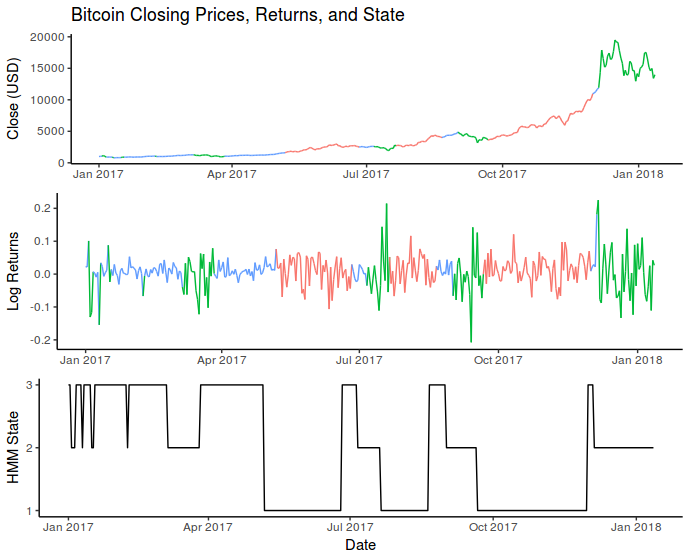
Below is a chart showing the most likely states during the 2017 and into the 2018 calendar years:
Here each of the three states are coloured. The blue state was characterized by positive average returns and low volatility. The red state also had generally positive returns but higher volatility. Finally, the green state had mostly negative returns and also high volatility.
I also ran a quick Shapiro-Wilk test on the log-valued daily returns which was unable to reject the null that daily returns come from a normal distribution. This means that there wasn’t enough evidence to disprove the assumption that price changes follow a Log-normal distribution.
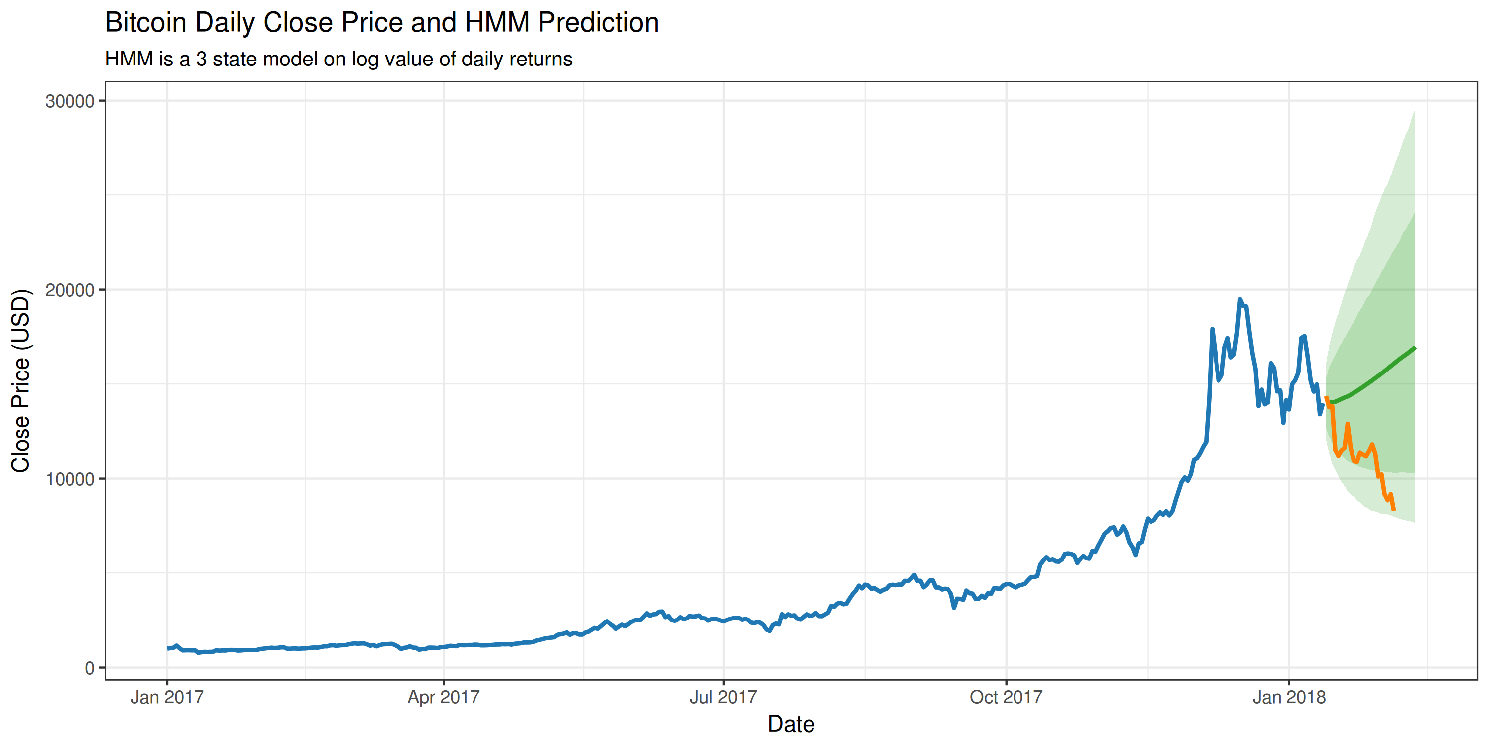
This is all fine and good, but what would be really cool is if the fitted model could be used to predict the future price of Bitcoin. So I ran 10,000 30-day simulations to get an expected future price and a confidence interval. This is what it looks like:
This shows the predicted Bitcoin price, and the actual price change during the prediction interval. The shaded regions also represent the 95% and 80% confidence intervals, based on the 10,000 simulations. In this instance, the HMM was not exactly a great predictor. Bitcoin has been incredibly volatile and I think it’s extremely difficult to make any meaningful predictions using closing price alone.
If you’re interested in taking a closer look at the R code used to fit the HMM model and generate the charts, you can find it on my Github.

